Training

The input represents the information and the weights represent the knowledge. Learning therefore means adjusting the weights so that the output corresponds to the expectations.

In supervised learning, the weights of the Artificial Neural Network ANN are iteratively adjusted so that the prediction comes as close as possible to the expected prediction.

For reasons of simplicity, the setting of the weight of a single artificial neuronal connection is shown here (Trask, 2019):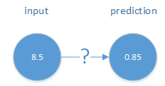

Setting the weight means learning

Because of the formula 

input * weight = prediction

you know immediately that the weight you are looking for must be 0.1: 

8.5 * 0.1 = 0.85 

Unfortunately, you cannot know the predictions of the hidden layers in deep artificial neural networks, so you have to calculate differently from back to front. The weight must be determined iteratively, i.e. approximately. The principle works as follows:

The untrained starting weight is determined (here 0). In a programme loop (20 iterations in this case), a prediction is made using the weight. The difference between this prediction and the actual prediction is then calculated. This difference is then weighted by multiplying it by the input value. This "weighted difference" is now multiplied by a learning rate (fixed here) and subtracted from the weight. The entire calculation is then repeated until the maximum number of repetitions is reached. In the optimum case, the weight is gradually adjusted better from iteration to iteration.

The following UML activity diagram illustrates this.

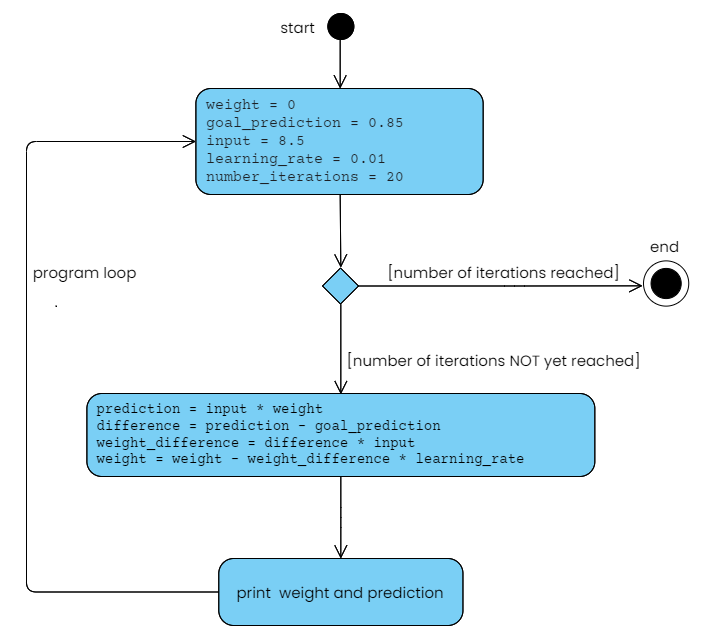
UML activity diagram of training of a single articial neural connection

Let's have a look at the 20 program outputs:

Difference: -0.85    Prediction: 0.0
Difference: -0.23587500000000006    Prediction: 0.6141249999999999 
Difference: -0.06545531249999992    Prediction: 0.7845446875000001 
Difference: -0.018163849218750028    Prediction: 0.83183615078125  
...
Difference: -2.9166857817841674e-10    Prediction: 0.8499999997083314
Difference: -8.093792303043301e-11    Prediction: 0.849999999919062
Difference: -2.246036689967923e-11    Prediction: 0.8499999999775396
End of program

The values for the weight and the prediction improve rapidly at first and then approach the optimum value more and more slowly. We could perhaps have made do with less accuracy in order to save computing time and energy. 

However, it is clear that no absolutely correct result can be achieved here. Only more or less accurate probabilities can be calculated.

It is also clear that the training process is much more computationally intensive than making predictions due to the high number of iterations.

Corresponding Python program:

 1   
 2
 3
 4
 5
 6
 7
 8
 9
10
11
12
13

weight = 0              # Start value of weight of untrained neural connection
goal_prediction = 0.85  
input = 8.5             
learning_rate = 0.01    # Adjust learning rate

for iteration in range(20):                             # 20 iterations
    prediction = input * weight                         # Calculate prediction
    difference = prediction - goal_prediction           # Difference from the expected result
    weight_difference = difference * input              # weight difference depending on the input value 
    weight = weight - weight_difference * learning_rate # Set new weight = learn with adjusted learning rate
    print("Difference: " + str(difference) + "    Prediction: " + str(prediction))

print("End of program")

Reference list:

Trask, Andrew W. (2019): Grokking Deep Learning. Chapter 4. Introduction to neural learning: gradient descent. Manning Publications Co.